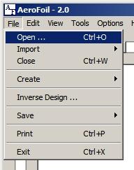
Calculations begin after selection of an airfoil. Airfoil coordinate data may be input from existing data files, input from a limited set of Drawing Interchange Files (.dxf), or read from raw x, y, and z coordinate files.

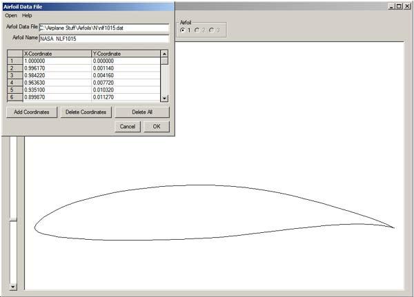
After the data file has been read it will be shown graphically on the main display and in a tabular grid. Coordinate points may be added, modified, or deleted as necessary. Some checks are performed on the data as it is being read and appropriate warning messages are displayed.

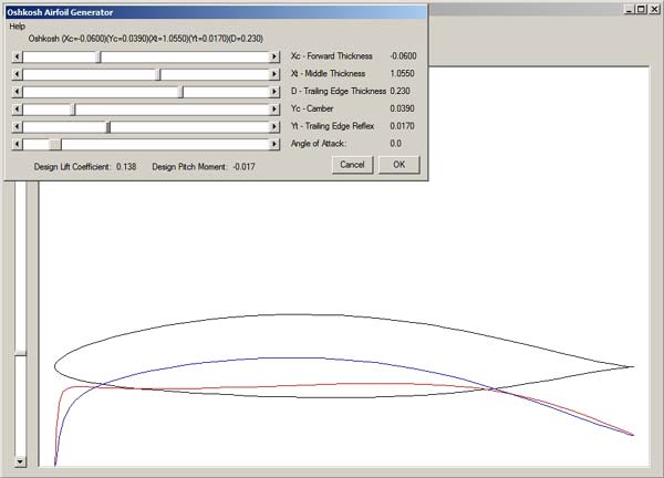
Airfoil coordinates may be generated using NACA methods

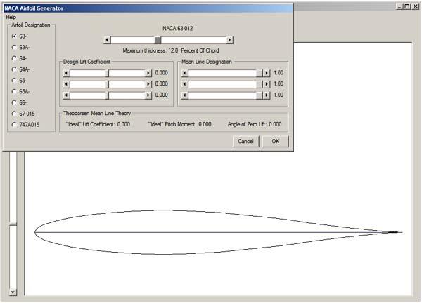
or using a simple, yet flexible, transformation model.

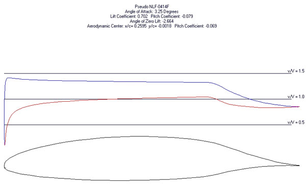
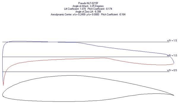
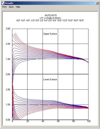
After selection of an airfoil, the calculations begin. The default display is velocity along the surface of the airfoil. The upper surface is shown in blue and the lower in red. The transition points from laminar to turbulent and flow separation are shown.

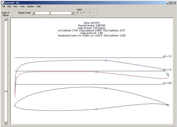
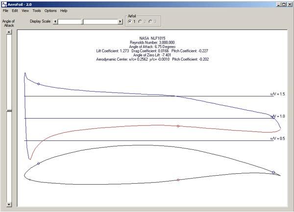
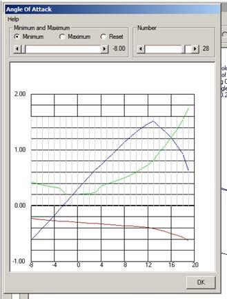
Use the Angle of Attack slider bar to show the effects at various angle of attack.

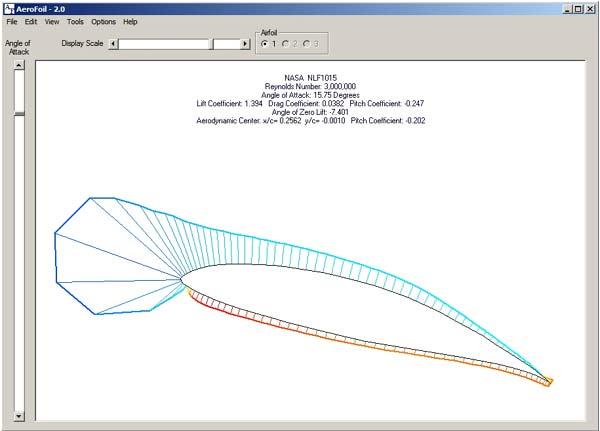
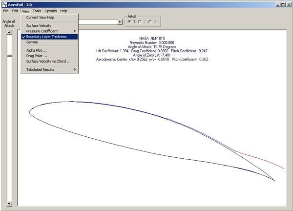
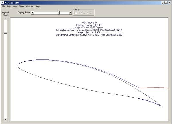
Switch to alternate views such as pressure coefficient or boundary layer thickness.

Use the Display Scale slider bar to increase or decrease the view of the selected parameter.

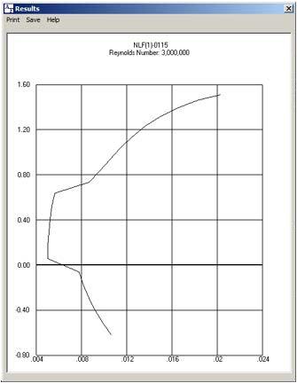
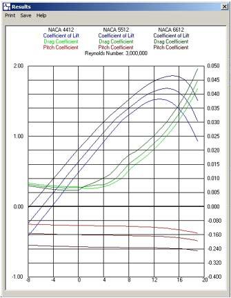
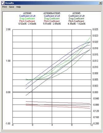
Select from different graphical displays such as lift, drag, and pitch vs angle of attack, drag vs lift, and velocity vs chord length

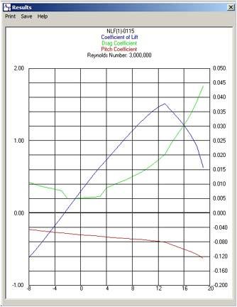
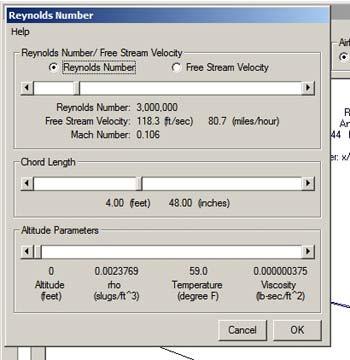
Change the calculations as necessary over a wide range of Reynolds Numbers and angles of attack.

A maximum of three different airfoils may be compared at one time.

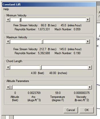
Not only are calculations performed at a constant Reynolds Number, but there are also two different simulations of an actual airfoil in real world conditions. In the simplest case, the total lift of the airfoil is held constant as the angle of attack is changed. This is what really happens to an airplane in flight.

In the more complex case, AeroFoil simulates a wing

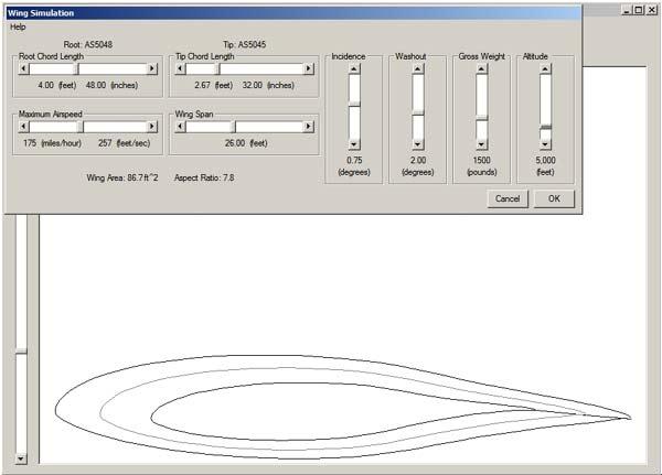
and calculates the performance characteristics at the root, mean aerodynamic chord, and tip.

Designing an airfoil using inverse modeling is a powerful way to create the most appropriate airfoil for a specific situation. During inverse modeling, a desired velocity profile is defined. All of the airfoil parameters such as maximum lift coefficient, angle of attack at stall, stall behavior, pitch moment, extent of laminar and turbulent flow, and the location of airflow separation are caused by the velocity profile. By specifying the desired velocity, an airfoil is created which will have the required performance.

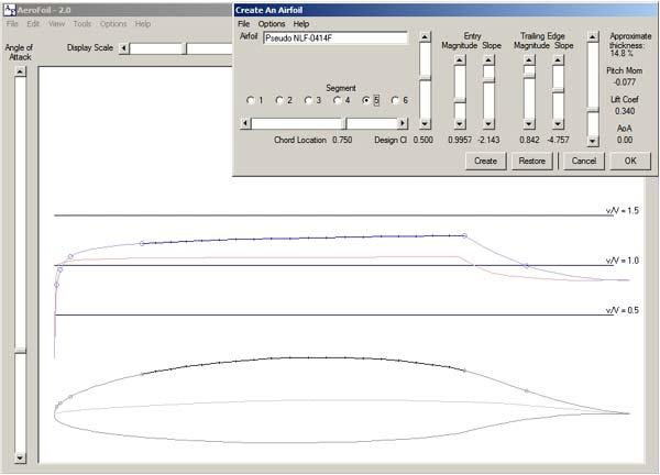
In the inverse modeling process, a segment of the airfoil is assigned a design coefficient of lift. On the upper surface of the airfoil, at any coefficient of lift less than this design value, the velocity over that segment will be increasing. This means that the boundary layer over that segment will remain attached to the surface and it will tend to remain laminar.

As the airfoil coefficient of lift increases above the design value over the segment, the velocity will begin to decrease. Boundary layer thickness will increase more rapidly, turbulent flow will begin to occur, which in turn will eventually result in airflow separation.

At the trailing edge, the shape of the velocity profile is altered just by adjusting the magnitude and slope. Boundary layer growth may be easily controlled. The design process may be exited at any time to allow any of the analysis calculations to be performed. Depending upon the results of the analysis calculations, the design process may be re-entered and changes made to the airfoil.

Go from one to another in just a few minutes.